sup_figure9

pkgs <- c("fs", "futile.logger", "configr", "stringr", "ggpubr", "ggthemes", 
          "SingleCellExperiment", "BiocNeighbors", "vroom", "jhtools", "glue", 
          "openxlsx", "ggsci", "patchwork", "cowplot", "tidyverse", "dplyr", 
          "survminer", "survival")
suppressMessages(conflicted::conflict_scout())
for (pkg in pkgs){
  suppressPackageStartupMessages(library(pkg, character.only = T))
}
res_dir <- "./results/sup_figure9" %>% checkdir
dat_dir <- "./data" %>% checkdir
config_dir <- "./config" %>% checkdir

#colors config
config_fn <- glue::glue("{config_dir}/configs.yaml")
stype3_cols <- jhtools::show_me_the_colors(config_fn, "stype3")
ctype10_cols <- jhtools::show_me_the_colors(config_fn, "cell_type_new")
meta_cols <- jhtools::show_me_the_colors(config_fn, "meta_color")
meta_merge_cols <- jhtools::show_me_the_colors(config_fn, "meta_merge")

#read in coldata
coldat <- readr::read_csv(glue::glue("{dat_dir}/sce_coldata.csv"))
sinfo <- readr::read_csv(glue::glue("{dat_dir}/metadata_sinfo.csv"))
sample_chemo_type_list <- readr::read_rds(glue::glue("{dat_dir}/sample_chemo_type_list.rds"))
metadata <- readr::read_rds(glue::glue("{dat_dir}/metadata.rds"))

grid.draw.ggsurvplot <- function(x){
  survminer:::print.ggsurvplot(x, newpage = FALSE)
}

sup_figure9a1

coldat <- coldat %>%
  dplyr::mutate(meta_merge = case_when(meta_cluster %notin% 
                                         c("MC-tumor-frontline", "MC-stroma-macro", "MC-tumor-core") ~ "MC-others",
                                       TRUE ~ meta_cluster))

#summary cell type prop
cell_type_meta3_total <- coldat %>% dplyr::filter(sample_id %in% sample_chemo_type_list$no_chemo_all) %>%
  group_by(sample_id, meta_merge) %>% summarise(nt = n()) %>% ungroup()

cell_type_meta3 <- coldat %>% dplyr::filter(sample_id %in% sample_chemo_type_list$no_chemo_all) %>%
  group_by(sample_id, cell_type_new, meta_merge) %>% summarise(nc = n()) %>% ungroup()

cell_type_meta3$cell_type_new <- factor(cell_type_meta3$cell_type_new)
cell_type_meta3 <- cell_type_meta3 %>%
  group_by(sample_id, meta_merge) %>%
  tidyr::complete(cell_type_new, fill = list(nc = 0)) %>% ungroup()
cell_type_meta3 <- left_join(cell_type_meta3_total, cell_type_meta3, by = c("sample_id", "meta_merge")) %>%
  dplyr::mutate(prop = nc/nt) %>% dplyr::select(-c(nt, nc)) %>% distinct()

#add os info
cell_type_meta3 <- left_join(cell_type_meta3, sinfo, by = "sample_id") %>%
  dplyr::select(sample_id, cell_type_new, meta_merge, prop, pfs_state, pfs_month, os_state, os_month)

#MC-stroma-macro
cell_type_meta3_sm <- cell_type_meta3 %>% dplyr::filter(cell_type_new == "HLA-DR-CD163- mp") %>%
  dplyr::filter(meta_merge == "MC-stroma-macro") %>%
  dplyr::mutate(group_mean = case_when(prop >= mean(prop) ~ "High DN-Mp (n = 54)", prop < mean(prop) ~ "Low DN-Mp (n = 60)"))

cell_type_meta3_sm_os <- cell_type_meta3_sm %>% dplyr::select(sample_id, os_state, os_month, group_mean) %>% drop_na(os_month)
cols <- c("High DN-Mp (n = 54)" = "#BC3C29FF", "Low DN-Mp (n = 60)" = "#0072B5FF")

#mean group
psurvx <- ggsurvplot(surv_fit(Surv(os_month, os_state) ~ group_mean, data = cell_type_meta3_sm_os), palette = cols,
                     legend.labs = levels(droplevels(as.factor(unlist(cell_type_meta3_sm_os[, "group_mean"])))),
                     size = 0.5, censor.size = 3, pval.size = 2,
                     pval = T, risk.table = F, xlim = c(0,75))
psurvx$plot <- psurvx$plot +
  guides(color=guide_legend(title="MC-stroma-Mp")) +
  theme(axis.title.y = element_text(size = 6),
        axis.text.y = element_text(size = 6),
        axis.title.x = element_text(size = 6),
        axis.text.x = element_text(size = 6),
        legend.text = element_text(size = 6),
        legend.title = element_text(size = 6),
        legend.position = c(0.7,0.75),
        legend.key.size = unit(0.1, 'cm'))
ggsave(glue::glue("{res_dir}/sup_figure9a1_DNmac_Stroma_Macro_os_mean.pdf"),
       plot = psurvx, width = 7, height = 7)
psurvx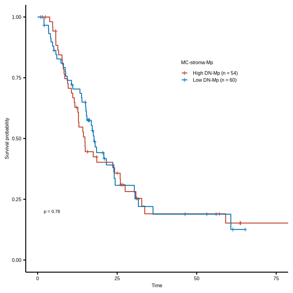

sup_figure9a2

#Other_metas
cell_type_meta3_oth <- cell_type_meta3 %>% dplyr::filter(cell_type_new == "HLA-DR-CD163- mp") %>%
  dplyr::filter(meta_merge == "MC-others") %>%
  dplyr::mutate(group_mean = case_when(prop >= mean(prop) ~ "High DN-Mp (n = 49)", 
                                       prop < mean(prop) ~ "Low DN-Mp (n = 96)"))

cell_type_meta3_oth_os <- cell_type_meta3_oth %>% 
  dplyr::select(sample_id, os_state, os_month, group_mean) %>% drop_na(os_month)
cols <- c("High DN-Mp (n = 49)" = "#BC3C29FF", "Low DN-Mp (n = 96)" = "#0072B5FF")

#mean group
psurvx <- ggsurvplot(surv_fit(Surv(os_month, os_state) ~ group_mean, data = cell_type_meta3_oth_os), palette = cols,
                     legend.labs = levels(droplevels(as.factor(unlist(cell_type_meta3_oth_os[, "group_mean"])))),
                     size = 0.5, censor.size = 3, pval.size = 2,
                     pval = T, risk.table = F, xlim = c(0,75))
psurvx$plot <- psurvx$plot +
  guides(color=guide_legend(title="MC-others")) +
  theme(axis.title.y = element_text(size = 6),
        axis.text.y = element_text(size = 6),
        axis.title.x = element_text(size = 6),
        axis.text.x = element_text(size = 6),
        legend.text = element_text(size = 6),
        legend.title = element_text(size = 6),
        legend.position = c(0.7,0.75),
        legend.key.size = unit(0.1, 'cm'))
ggsave(glue::glue("{res_dir}/sup_figure9a2_DNmac_Other_metas_os_mean.pdf"),
       plot = psurvx, width = 7, height = 7)
psurvx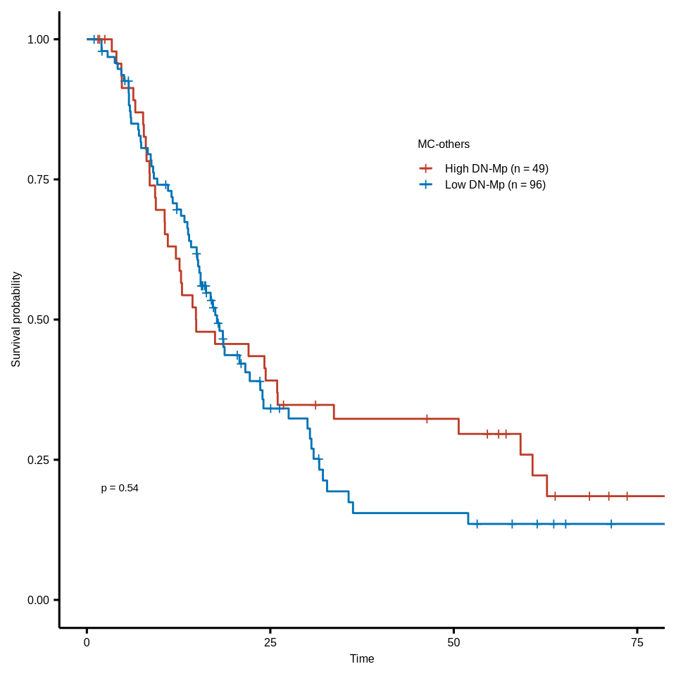

sup_figure9b

#summary cell type prop
cell_type_total <- coldat %>% dplyr::filter(sample_id %in% sample_chemo_type_list$no_chemo_all) %>%
  group_by(sample_id, cell_type_new) %>% summarise(nc = n()) %>%
  group_by(sample_id) %>% dplyr::mutate(nt = sum(nc)) %>% ungroup() %>%
  dplyr::mutate(prop = nc/nt)

cell_type_total$cell_type_new <- factor(cell_type_total$cell_type_new)
cell_type_total <- cell_type_total %>%
  group_by(sample_id) %>%
  tidyr::complete(cell_type_new, fill = list(prop = 0)) %>% ungroup()

cell_type_dnmac <- cell_type_total %>% dplyr::filter(cell_type_new == "HLA-DR-CD163- mp")

cell_type_dnmac <- left_join(cell_type_dnmac, sinfo, by = "sample_id") %>%
  dplyr::select(sample_id, prop, os_state, os_month)

cell_type_dnmac <- cell_type_dnmac %>%
  dplyr::mutate(group_mean = case_when(prop >= mean(prop) ~ "High DN-Mp (n = 57)", 
                                       prop < mean(prop) ~ "Low DN-Mp (n = 89)")) %>% 
  drop_na(os_month)

cols <- c("High DN-Mp (n = 57)" = "#BC3C29FF", "Low DN-Mp (n = 89)" = "#0072B5FF")

#mean group
psurvx <- ggsurvplot(surv_fit(Surv(os_month, os_state) ~ group_mean, data = cell_type_dnmac), palette = cols,
                     legend.labs = levels(droplevels(as.factor(unlist(cell_type_dnmac[, "group_mean"])))),
                     size = 0.5, censor.size = 3, pval.size = 2,
                     pval = T, risk.table = F, xlim = c(0,75))
psurvx$plot <- psurvx$plot +
  guides(color=guide_legend(title="Total ROI")) +
  theme(axis.title.y = element_text(size = 6),
        axis.text.y = element_text(size = 6),
        axis.title.x = element_text(size = 6),
        axis.text.x = element_text(size = 6),
        legend.text = element_text(size = 6),
        legend.title = element_text(size = 6),
        legend.position = c(0.7,0.75),
        legend.key.size = unit(0.1, 'cm'))
ggsave(glue::glue("{res_dir}/sup_figure9b_DNmac_total_region_os_mean.pdf"),
       plot = psurvx, width = 7, height = 7)
psurvx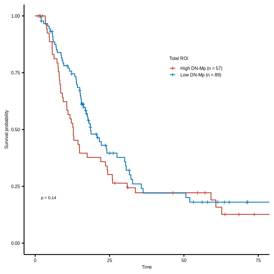

sup_figure9c

#CD8T in TB prop OS
CD8T_meta3_tb <- cell_type_meta3 %>% dplyr::filter(cell_type_new == "CD8+ T cell") %>%
  dplyr::filter(meta_merge == "MC-tumor-frontline") %>%
  dplyr::mutate(group_mean = case_when(prop >= mean(prop) ~ "High CD8+ T cell (n = 39)", 
                                       prop < mean(prop) ~ "Low CD8+ T cell (n = 92)"))

CD8T_meta3_tb_os <- CD8T_meta3_tb %>% dplyr::select(sample_id, os_state, os_month, group_mean) %>% drop_na(os_month)
cols <- c("High CD8+ T cell (n = 39)" = "#BC3C29FF", "Low CD8+ T cell (n = 92)" = "#0072B5FF")

#mean group
psurvx <- ggsurvplot(surv_fit(Surv(os_month, os_state) ~ group_mean, data = CD8T_meta3_tb_os), palette = cols,
                     legend.labs = levels(droplevels(as.factor(unlist(CD8T_meta3_tb_os[, "group_mean"])))),
                     size = 0.5, censor.size = 3, pval.size = 2,
                     pval = T, risk.table = F, xlim = c(0,75))
psurvx$plot <- psurvx$plot +
  guides(color=guide_legend(title="MC-tumor-frontline")) +
  theme(axis.title.y = element_text(size = 6),
        axis.text.y = element_text(size = 6),
        axis.title.x = element_text(size = 6),
        axis.text.x = element_text(size = 6),
        legend.text = element_text(size = 6),
        legend.title = element_text(size = 6),
        legend.position = c(0.7,0.75),
        legend.key.size = unit(0.1, 'cm'))
ggsave(glue::glue("{res_dir}/sup_figure9c_CD8T_Tumor_boundary_os_mean.pdf"),
       plot = psurvx, width = 7, height = 7)
psurvx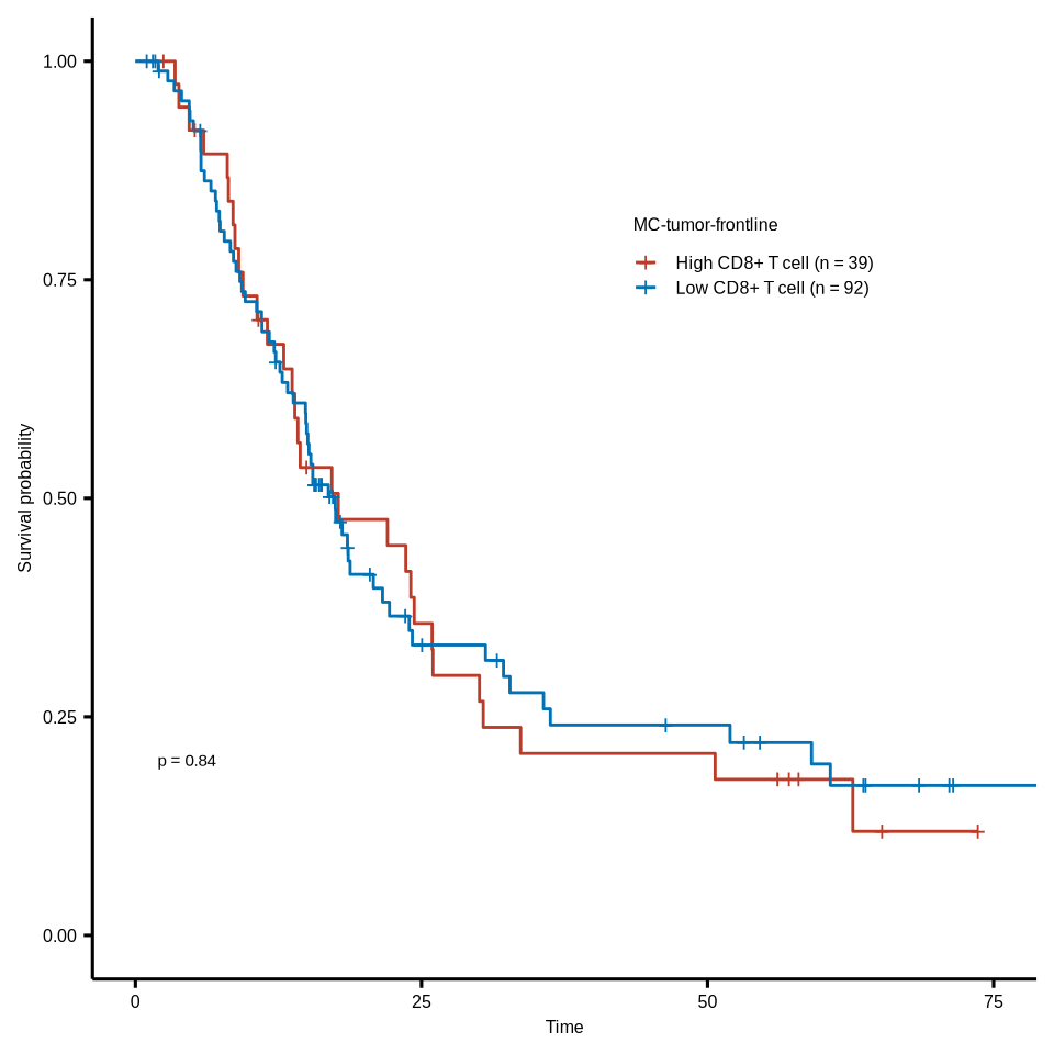

sup_figure9d

ctype_prop_3metas <- coldat %>% dplyr::filter(sample_id %in% sample_chemo_type_list$no_chemo_all & 
                                                meta_merge != "MC-tumor-core") %>%
  dplyr::select(sample_id, cell_type_new, meta_merge) %>% group_by(sample_id, cell_type_new, meta_merge) %>%
  dplyr::mutate(nc = n()) %>% ungroup() %>% distinct() %>%
  group_by(sample_id, meta_merge) %>%
  dplyr::mutate(nt = sum(nc),
                prop = nc/nt) %>% ungroup()

ctype_prop_3metas$meta_merge <- factor(ctype_prop_3metas$meta_merge, 
                                       levels = c("MC-tumor-frontline", "MC-stroma-macro", "MC-others"))
ctype_prop_3metas$cell_type_new <- factor(ctype_prop_3metas$cell_type_new)
ctype_prop_3metas <- ctype_prop_3metas %>%
  group_by(sample_id, meta_merge) %>%
  complete(cell_type_new, fill = list(prop = 0, nc = 0)) %>%
  tidyr::fill(nt, .direction = "downup") %>% ungroup()


#DNmac prop in 3 metas
dat_plot <- ctype_prop_3metas %>% dplyr::filter(cell_type_new == "HLA-DR-CD163- mp")
#quantile(dat_plot$prop, prob = 0.9) %>% as.numeric()
dat_plot$meta_merge <- as.character(dat_plot$meta_merge)

dat_plot$meta_merge <- factor(dat_plot$meta_merge, levels = c("MC-tumor-frontline", "MC-stroma-macro", "MC-others"))
my_comparisons <- list(c("MC-tumor-frontline", "MC-stroma-macro"), c("MC-stroma-macro", "MC-others"), c("MC-tumor-frontline", "MC-others"))

stat_test <- dat_plot %>% rstatix::wilcox_test(prop ~ meta_merge, comparisons = my_comparisons)
stat_test$y.position <- c(0.45,0.43,0.41)

dat_plot$prop[dat_plot$prop > quantile(dat_plot$prop, prob = 0.95)] <- quantile(dat_plot$prop, prob = 0.95)
dat_plot <- dat_plot %>% group_by(meta_merge, cell_type_new) %>% dplyr::mutate(ng = n()) %>% ungroup

p <- ggplot(dat_plot,
            aes(x = meta_merge, y = prop)) +
  geom_boxplot(aes(fill = meta_merge), width = .3, show.legend = FALSE,
               outlier.shape = NA, linewidth = .2, color = "black") +
  stat_summary(aes(fill = meta_merge, color = meta_merge), fun.data = "mean_se", geom = "pointrange", show.legend = F,
               position = position_dodge(.5), fatten = .5, size = .5, stroke = .5, linewidth = .5, color = "black") +
  #scale_y_continuous(limits=c(0,0.4), oob = scales::rescale_none) +
  ylim(0,0.45) + ylab(glue::glue("Proportion of DN-Mp")) +
  scale_fill_manual(values = meta_merge_cols) +
  stat_pvalue_manual(stat_test, tip.length = .03, bracket.size = 0.2, label = "p.adj.signif", size = 2) +
  directlabels::geom_dl(aes(label = ng), method = list("top.points", cex = .4)) +
  theme_bmbdc() +
  theme(title = element_text(size = 6),
        axis.ticks = element_line(colour = "black"),
        axis.title.y = element_text(size = 6),
        axis.text.y = element_text(size = 6, colour = "black"),
        axis.title.x = element_blank(),
        axis.text.x = element_text(size = 6, colour = "black", angle = 10),
        axis.line.x = element_line(linewidth = 0.4),
        axis.line.y = element_line(linewidth = 0.4),
        legend.position="none")
ggsave(glue::glue("{res_dir}/sup_figure9d_DNmac_prop_3metas_only.pdf"), p, width = 3, height = 3)
p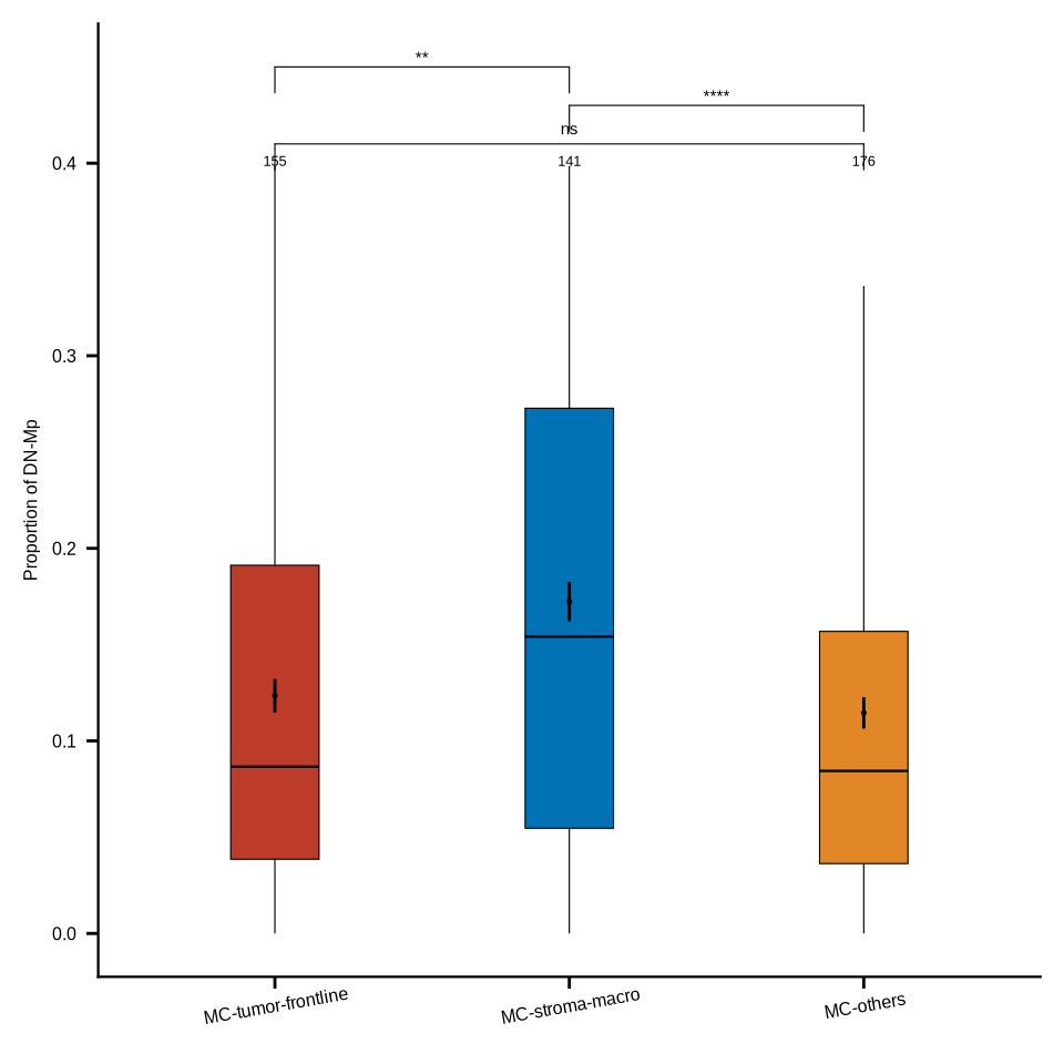

sup_figure9e

coldat <- coldat %>%
  dplyr::mutate(cell_type11 = case_when(cell_type_new %in%
                                          c("HLA-DR+CD163- mp", "HLA-DR+CD163+ mp", "HLA-DR-CD163+ mp") ~ "Other-mp",
                                        cell_type_new %in% c("HLA-DR-CD163- mp") ~ "DN-mp",
                                        TRUE ~ cell_type_new))

DNmac_TB_prop <- coldat %>%
  group_by(sample_tiff_id, meta_merge, cell_type11) %>%
  dplyr::summarise(nc = n()) %>% group_by(sample_tiff_id, meta_merge) %>%
  dplyr::mutate(nt = sum(nc)) %>% ungroup() %>%
  dplyr::mutate(prop = nc/nt) %>%
  dplyr::filter(meta_merge == "MC-tumor-frontline")
DNmac_TB_prop$cell_type11 <- factor(DNmac_TB_prop$cell_type11)
DNmac_TB_prop <- DNmac_TB_prop %>% group_by(sample_tiff_id) %>%
  tidyr::complete(cell_type11, fill = list(prop = 0)) %>% ungroup() %>%
  distinct() %>% dplyr::filter(cell_type11 == "DN-mp")

#tiffs have TB and SM
TB_SM_tiffs <- coldat[, c("sample_tiff_id", "meta_cluster")] %>% distinct() %>%
  drop_na(meta_cluster) %>% dplyr::mutate(exist = 1) %>%
  pivot_wider(names_from = meta_cluster, values_from = exist, values_fill = 0) %>%
  dplyr::filter(`MC-tumor-frontline` != 0 & `MC-stroma-macro` != 0) %>% .$sample_tiff_id %>% unique()

df_inter_weighted <- metadata[["community_interaction_weighted"]] %>%
  dplyr::filter(from_meta != to_meta) %>%
  dplyr::mutate(inter_pair =
                  case_when(from_meta == "MC-tumor-frontline" & to_meta == "MC-stroma-macro" ~ "TB_SM",
                            from_meta == "MC-stroma-macro" & to_meta == "MC-tumor-frontline" ~ "TB_SM",
                            from_meta == "MC-tumor-frontline" & to_meta != "MC-stroma-macro" ~ "TB_Others",
                            from_meta != "MC-stroma-macro" & to_meta == "MC-tumor-frontline" ~ "TB_Others",
                            TRUE ~ "Others")) %>%
  dplyr::filter(inter_pair != "Others") %>%
  dplyr::filter(sample_tiff_id %in% TB_SM_tiffs)

df_inter_weighted_mean <- df_inter_weighted %>%
  group_by(sample_tiff_id, inter_pair) %>%
  summarise(mean_wt = mean(weight)) %>% ungroup()
df_inter_weighted_mean <- df_inter_weighted_mean %>%
  tidyr::complete(sample_tiff_id, inter_pair, fill = list(mean_wt = 0))

data_df <- left_join(df_inter_weighted_mean[df_inter_weighted_mean$inter_pair == "TB_SM",],
                     DNmac_TB_prop,
                     by = "sample_tiff_id")

cor_res <- data.frame("cor" = cor.test(formula = ~ mean_wt + prop,
                                       data = data_df)$estimate,
                      "pval" = cor.test(formula = ~ mean_wt + prop,
                                        data = data_df)$p.value)

p <- ggscatter(data_df, x = "mean_wt", y = "prop",
               palette = "#BC3C29FF", size = .01,
               add = "reg.line", conf.int = TRUE, star.plot.lwd = .1,
               cor.coef.size = .01) + xlim(0,1) +
  scale_x_continuous(limits=c(0,20), oob = scales::rescale_none) +
  xlab(glue::glue("Mean weight of interaction")) + ylab(glue::glue("Proportion of DN-Mp")) +
  stat_cor(aes(color = "#BC3C29FF"), label.x = 11, size = 3) +
  theme(axis.title.y = element_text(size = 6),
        axis.text.y = element_text(size = 6),
        axis.title.x = element_text(size = 6),
        axis.text.x = element_text(size = 6),
        legend.position = "none")
ggsave(glue::glue("{res_dir}/sup_figure9e_correlation_TBSMinteractionWT_DNmacpropTB.pdf"), p, width = 5, height = 5)
p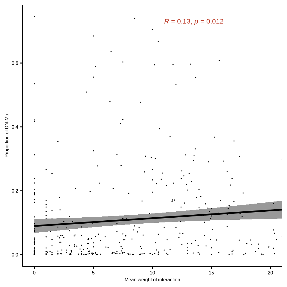

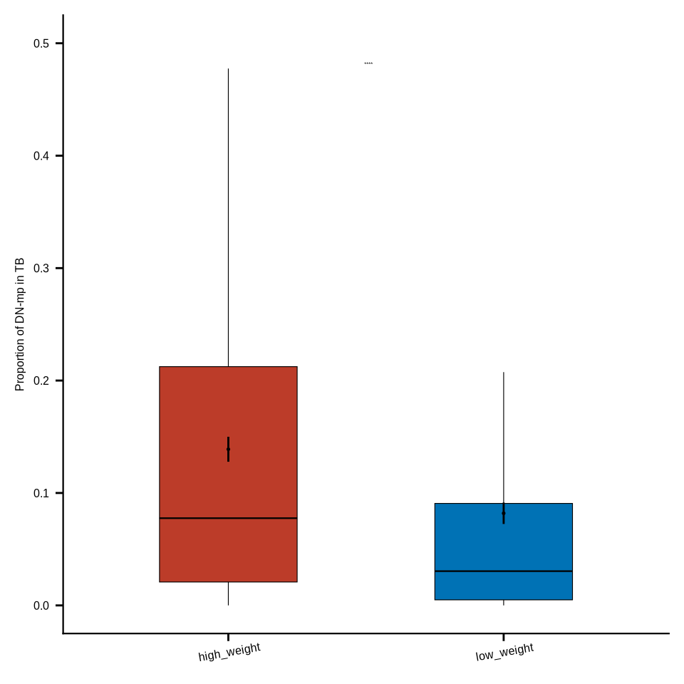
sup_figure9f

DNmac_TB_prop <- coldat %>%
  group_by(sample_tiff_id, meta_merge, cell_type11) %>%
  dplyr::summarise(nc = n()) %>% group_by(sample_tiff_id, meta_merge) %>%
  dplyr::mutate(nt = sum(nc)) %>% ungroup() %>%
  dplyr::mutate(prop = nc/nt) %>%
  dplyr::filter(meta_merge == "MC-tumor-frontline")
DNmac_TB_prop$cell_type11 <- factor(DNmac_TB_prop$cell_type11)
DNmac_TB_prop <- DNmac_TB_prop %>% group_by(sample_tiff_id) %>%
  tidyr::complete(cell_type11, fill = list(prop = 0)) %>% ungroup() %>%
  distinct() %>% dplyr::filter(cell_type11 == "DN-mp")

#tiffs have TB and SM
TB_SM_tiffs <- coldat[, c("sample_tiff_id", "meta_cluster")] %>% distinct() %>%
  drop_na(meta_cluster) %>% dplyr::mutate(exist = 1) %>%
  pivot_wider(names_from = meta_cluster, values_from = exist, values_fill = 0) %>%
  dplyr::filter(`MC-tumor-frontline` != 0 & `MC-stroma-macro` != 0) %>% .$sample_tiff_id %>% unique()

df_inter_weighted <- metadata[["community_interaction_weighted"]] %>%
  dplyr::filter(from_meta != to_meta) %>%
  dplyr::mutate(inter_pair =
                  case_when(from_meta == "MC-tumor-frontline" & to_meta == "MC-stroma-macro" ~ "TB_SM",
                            from_meta == "MC-stroma-macro" & to_meta == "MC-tumor-frontline" ~ "TB_SM",
                            from_meta == "MC-tumor-frontline" & to_meta != "MC-stroma-macro" ~ "TB_Others",
                            from_meta != "MC-stroma-macro" & to_meta == "MC-tumor-frontline" ~ "TB_Others",
                            TRUE ~ "Others")) %>%
  dplyr::filter(inter_pair != "Others") %>%
  dplyr::filter(sample_tiff_id %in% TB_SM_tiffs)

df_inter_weighted_mean <- df_inter_weighted %>%
  group_by(sample_tiff_id, inter_pair) %>%
  summarise(mean_wt = mean(weight)) %>% ungroup()
df_inter_weighted_mean <- df_inter_weighted_mean %>%
  tidyr::complete(sample_tiff_id, inter_pair, fill = list(mean_wt = 0))

data_df <- left_join(df_inter_weighted_mean[df_inter_weighted_mean$inter_pair == "TB_SM",],
                     DNmac_TB_prop,
                     by = "sample_tiff_id")

data_df <- data_df %>% dplyr::select(sample_tiff_id, mean_wt, prop) %>%
  dplyr::mutate(group_md = case_when(mean_wt >= median(mean_wt) ~ "high_weight", mean_wt < median(mean_wt) ~ "low_weight"))

col_d <- c("high_weight" = "#BC3C29FF", "low_weight" = "#0072B5FF")

p <- ggplot(data_df,
              aes(x = group_md, y = prop)) +
    geom_boxplot(aes(fill = group_md), width = .5, show.legend = FALSE,
                 outlier.shape = NA, linewidth = .2, color = "black") +
    stat_summary(aes(fill = group_md, color = group_md), fun.data = "mean_se", geom = "pointrange", show.legend = F,
                 position = position_dodge(.5), fatten = .5, size = .5, stroke = .5, linewidth = .5, color = "black") +
    scale_colour_manual(values = col_d) +
    scale_fill_manual(values = col_d) +
    labs(y = "Proportion of DN-mp in TB") +
    stat_compare_means(aes(label = after_stat(p.signif)), label.y = 0.48,
                       tip.length = 0, label.x.npc = "center",
                       method = "wilcox.test", size = 1) +
    scale_y_continuous(limits=c(0,0.5), oob = scales::rescale_none) +
    theme_bmbdc() +
    theme(title = element_text(size = 6),
          axis.ticks = element_line(colour = "black"),
          axis.title.y = element_text(size = 6),
          axis.text.y = element_text(size = 6, colour = "black"),
          axis.title.x = element_blank(),
          axis.text.x = element_text(size = 6, colour = "black", angle = 10),
          axis.line.x = element_line(linewidth = 0.4),
          axis.line.y = element_line(linewidth = 0.4),
          legend.position="top",
          legend.text = element_text(size = 4),
          legend.title = element_text(size = 4),
          legend.key.size = unit(0.1, 'cm'))
ggsave(glue::glue("{res_dir}/sup_figure9f_TB_SM_DNmac_prop_group_md.pdf"), p, height = 3, width = 1.5)
p