pkgs <- c("fs", "futile.logger", "configr", "stringr", "ggpubr", "ggthemes", "clusterProfiler",
          "vroom", "jhtools", "glue", "openxlsx", "ggsci", "patchwork", "cowplot",
          "tidyverse", "dplyr", "Seurat", "harmony", "ggpubr", "GSVA", "EnhancedVolcano")
suppressMessages(conflicted::conflict_scout())
for (pkg in pkgs){
  suppressPackageStartupMessages(library(pkg, character.only = T))
}
res_dir <- "./results/sup_figure14" %>% checkdir
dat_dir <- "./data" %>% checkdir
config_dir <- "./config" %>% checkdir

#colors config
config_fn <- glue::glue("{config_dir}/configs.yaml")
rctd_cols <- jhtools::show_me_the_colors(config_fn, "rctd_colors")

#read in coldata
sce_mac <- read_rds(glue::glue("{dat_dir}/sce_mac_DNp50_retsne.rds"))
spatial_mac_tumor <- read_rds(glue::glue("{dat_dir}/spatial_mac_tumor.rds"))sup_figure14
sup_figure14b
pl <- list()
for (i in c("S100A9", "RPL17", "DUSP6", "CDC42EP3")) {
  pdf(glue::glue("{res_dir}/sfig14b_sce_mac_{i}_exp_featureplot.pdf"), width = 2.5, height = 2)
  pl[[i]] <- FeaturePlot(sce_mac, reduction = "tsne", features = i,
                   order = F, pt.size = .001, combine = F)
  pl[[i]] <- pl[[i]][[1]] +
    guides(color = guide_colourbar(barwidth = unit(.1, "cm"),
                                   barheight = unit(.6, "cm"),
                                   title = i,
                                   title.position = "top")) +
    theme(plot.title = element_blank(),
          axis.text = element_blank(),
          axis.title = element_text(size = 8),
          axis.line = element_blank(),
          axis.ticks = element_blank(),
          panel.spacing = unit(0, "mm"),
          panel.border = element_rect(fill = NA, colour = NA),
          plot.background = element_rect(fill = NA, colour = NA),
          plot.margin = margin(0,0,0,0),
          legend.position = c(0,.8),
          legend.margin = margin(0,0,0,0),
          legend.title = element_text(size = 6),
          legend.text = element_text(size = 6))
  print(pl[[i]])
  dev.off()
}
pl[[1]] | pl[[2]] | pl[[3]] | pl[[4]]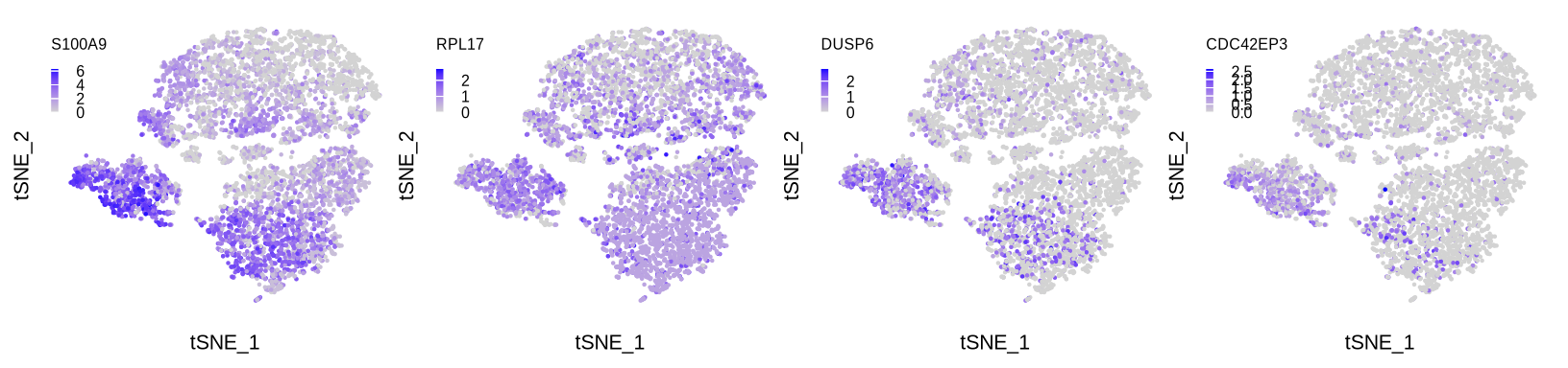
sup_figure14c
sce_mac$cell_types2 <- factor(sce_mac$cell_types2, levels = c("DN-mp", "Other-mp"))
Idents(sce_mac) <- "cell_types2"
#pdf(glue::glue("{res_dir}/sfig14c_sce_mac_S100A9_vlnplot.pdf"), width = 3, height = 3)
p <- VlnPlot(sce_mac, features = "S100A9", pt.size = 0,
             cols = c("DN-mp" = "#BC3C29FF", "Other-mp" = "#0072B5FF"), combine = F)
p <- p[[1]] + ylab("S100A9") +
  theme(plot.title = element_blank(),
        axis.text = element_text(size = 6),
        axis.title.y = element_text(size = 8, margin = margin(0,0,0,0)),
        axis.title.x = element_blank(),
        axis.text.x = element_text(size = 8, angle = 10),
        axis.line.x = element_line(linewidth = 0.4),
        axis.line.y = element_line(linewidth = 0.4),
        legend.text=element_text(size = 4),
        legend.key.size = unit(.2, "cm"))
print(p)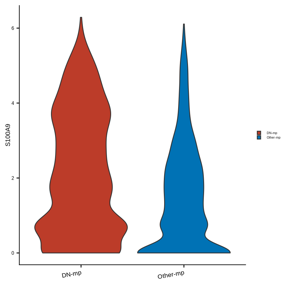
sup_figure14d
spatial_mac_tumor$DN_any <- factor(spatial_mac_tumor$DN_any, levels = c("DN-mac enriched", "Other-mac enriched"))
Idents(spatial_mac_tumor) <- "DN_any"

#pdf(glue::glue("{res_dir}/sfig14d_seu_mactumor_s100a9.pdf"), width = 3, height = 3)
p <- VlnPlot(spatial_mac_tumor, features = "S100A9", pt.size = 0, combine = F,
             cols = c("DN-mac enriched" = "#BC3C29FF", "Other-mac enriched" = "#0072B5FF"))
p <- p[[1]] + ylab("S100A9") +
  theme(plot.title = element_blank(),
        axis.text = element_text(size = 6),
        axis.title.y = element_text(size = 8),
        axis.title.x = element_blank(),
        axis.text.x = element_text(size = 8, angle = 10),
        axis.line.x = element_line(linewidth = 0.4),
        axis.line.y = element_line(linewidth = 0.4),
        legend.text=element_text(size = 4),
        legend.key.size = unit(.2, "cm"))
print(p)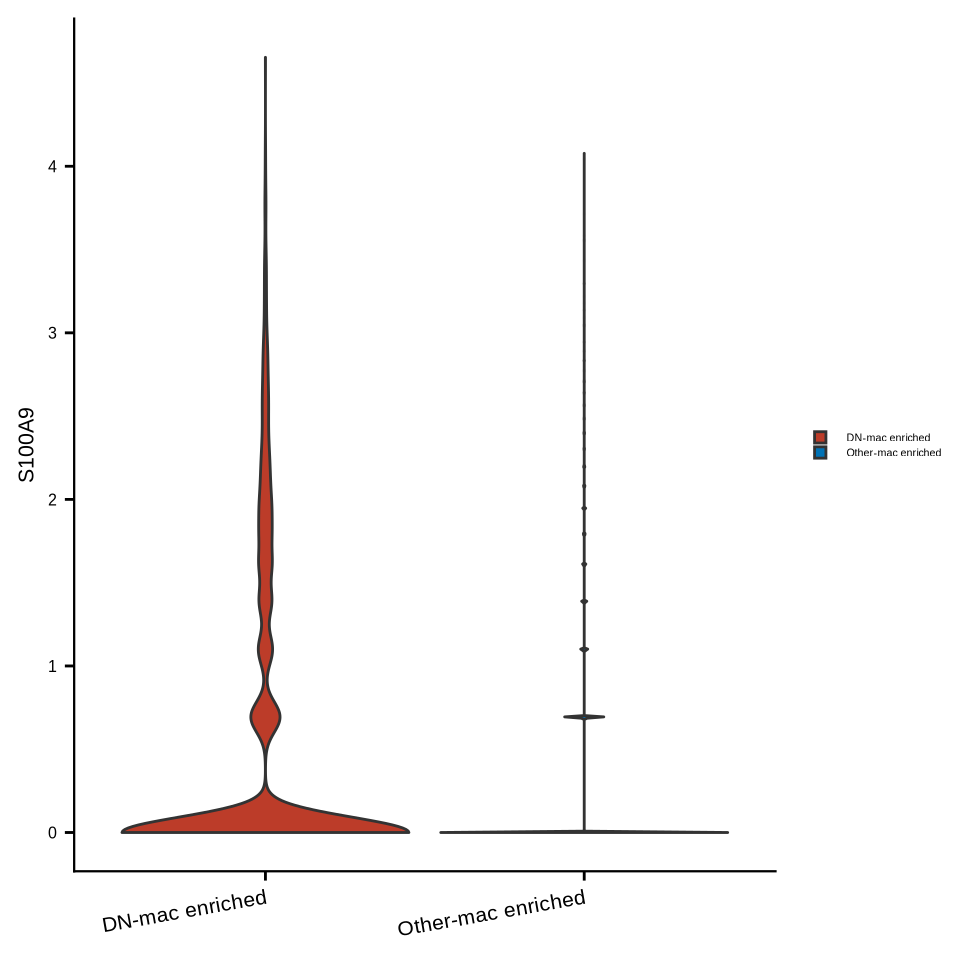
sup_figure14e
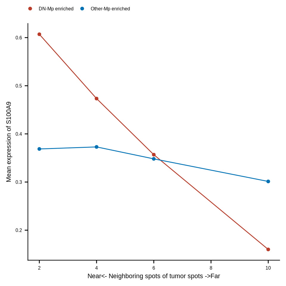
df_k_exp <- read_csv(glue::glue("{dat_dir}/df_knn_exp.csv"))

df_k_exp_dnm <- df_k_exp %>%
  dplyr::mutate(DN_any = case_when(CD68 > 0 & if_any(contains("HLA"), ~ .x == 0) &
                                     CD163 == 0 ~ "DN-Mp enriched",
                                   CD68 == 0 ~ "NoMp_enriched",
                                   TRUE ~ "Other-Mp enriched"))

df_spotmac <- df_k_exp_dnm %>% dplyr::filter(DN_any != "NoMp_enriched")

df_spotmac_mean <- df_spotmac %>% group_by(k, DN_any) %>%
  dplyr::transmute(across(CD68:S100A9, mean, .names = "mean_{.col}")) %>%
  ungroup() %>% distinct() %>% pivot_longer(cols = mean_CD68:mean_S100A9, names_to = "gene", values_to = "exp")

p <- ggplot(df_spotmac_mean[df_spotmac_mean$gene == "mean_S100A9" & df_spotmac_mean$k != 0,],
            aes(x=k, y=exp, color=DN_any, group = DN_any)) +
  geom_point() + geom_line() + xlab("k") + ylab(glue::glue("Mean expression of S100A9")) +
  scale_color_manual(values=c("DN-Mp enriched" = "#BC3C29FF", "Other-Mp enriched" = "#0072B5FF")) +
  xlab("Near<- Neighboring spots of tumor spots ->Far") +
  theme_bmbdc() +
  theme(plot.title = element_blank(),
        plot.subtitle = element_blank(),
        text = element_text(size = 6),
        axis.text = element_text(size = 6),
        axis.title.x = element_text(size = 8),
        axis.title.y = element_text(size = 8),
        axis.line.x = element_line(linewidth = 0.4),
        axis.line.y = element_line(linewidth = 0.4),
        legend.key.size = unit(.2, 'cm'),
        legend.title = element_blank(),
        legend.text = element_text(size=6),
        legend.position = "top")
ggsave(glue::glue("{res_dir}/sfig14e_visium_spotmac_mean_s100a9_k24610.pdf"), p, width = 3, height = 3.3)
p