pkgs <- c("fs", "futile.logger", "configr", "stringr", "ggpubr", "ggthemes",
          "vroom", "jhtools", "glue", "openxlsx", "ggsci", "patchwork", "cowplot",
          "tidyverse", "dplyr", "SingleCellExperiment", "survminer", "survival")
suppressMessages(conflicted::conflict_scout())
for (pkg in pkgs){
  suppressPackageStartupMessages(library(pkg, character.only = T))
}
res_dir <- "./results/figure7" %>% checkdir
dat_dir <- "./data" %>% checkdir
config_dir <- "./config" %>% checkdir

#colors config
config_fn <- glue::glue("{config_dir}/configs.yaml")
stype3_cols <- jhtools::show_me_the_colors(config_fn, "stype3")
ctype10_cols <- jhtools::show_me_the_colors(config_fn, "cell_type_new")

#read in coldata
coldat <- readr::read_csv(glue::glue("{dat_dir}/sce_coldata.csv"))
ph_df_markers_norm <- readr::read_csv(glue::glue("{dat_dir}/polaris_markers_norm.csv"))figure7
figure7d
#hyperion size
hyperion_comsize_su <- coldat %>% dplyr::filter(stype2 %in% c("tumor", "after_chemo")) %>%
  na.omit() %>% group_by(community_name) %>%
  summarise(n = n())

#polaris size
dt_cl <- readr::read_csv(glue::glue("{dat_dir}/cell_community_neighbors32res12.csv"))
#plot of community size compare
comsize_su_com <- rbind(dt_cl %>% drop_na(community) %>% dplyr::select(community_id, n) %>%
                          distinct() %>% dplyr::mutate(group = "polaris"),
                        hyperion_comsize_su %>% dplyr::rename(community_id = community_name) %>%
                          dplyr::mutate(group = "hyperion"))

p1 <- ggdensity(comsize_su_com, x = "n", xlab = "community size",
                add = "mean", rug = F,
                color = "group", fill = "group",
                palette = ggsci::pal_nejm("default")(2)) +
  theme(axis.title.y = element_text(size = 6),
        axis.text.y = element_text(size = 6),
        axis.title.x = element_text(size = 6),
        axis.text.x = element_text(size = 6),
        axis.line.x = element_line(linewidth = 0.4),
        axis.line.y = element_line(linewidth = 0.4),
        legend.position = c(.7, .7),
        legend.text = element_text(size = 6),
        legend.title = element_blank(),
        legend.key.size = unit(0.2, 'cm'))
ggsave(glue::glue("{res_dir}/fig7d_hyperion_polaris231031_community_size_compare_neighbors32res12.pdf"), p1, height = 3, width = 3)
p1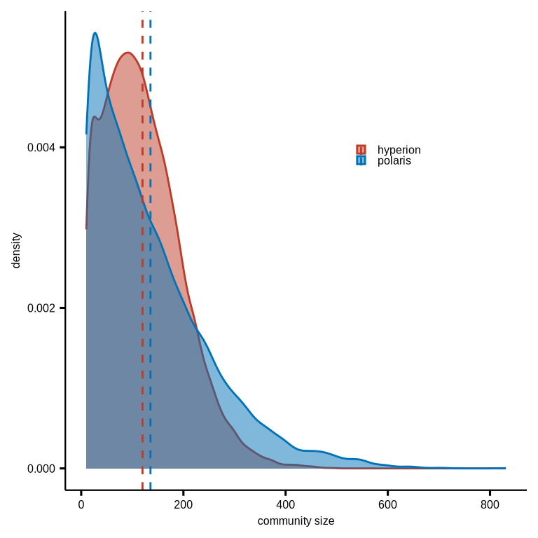
figure7e
mac_markers <- ph_df_markers_norm %>% dplyr::filter(phenotype %in% c("DN_macrophage", "Other_macrophage"))

mac_mean <- mac_markers %>% group_by(roi_id, phenotype) %>%
  dplyr::summarise(across(Pan_CK:CD163, ~ mean(.x))) %>% ungroup() %>%
  dplyr::mutate(phenotype = case_match(phenotype,
                                       "DN_macrophage" ~ "DN-Mp",
                                       "Other_macrophage" ~ "Other-Mp"))
mac_mean_df <- mac_mean %>% pivot_longer(cols = Pan_CK:CD163, names_to = "markers", values_to = "intensity")

mac_mean_df$phenotype <- factor(mac_mean_df$phenotype, levels = c("DN-Mp", "Other-Mp"))
mac_mean_df$markers <- factor(mac_mean_df$markers, levels = c("Pan_CK", "a_SMA", "CD68", "HLA_DR", "CD163", "S100A9"))

stat_test <- mac_mean_df %>%
  group_by(markers) %>% rstatix::wilcox_test(intensity ~ phenotype, paired = F)
stat_test <- stat_test %>% mutate(p.adj.signif = case_when(p >= 0.05 ~ "ns",
                                                           p >= 0.01 & p < 0.05 ~ "*",
                                                           p >= 0.001 & p < 0.01 ~ "**",
                                                           p >= 0.0001 & p < 0.001 ~ "***",
                                                           p < 0.0001 ~ "****",
                                                           TRUE ~ "ns"))
stat_test <- stat_test %>%
  rstatix::add_xy_position(x = "markers", dodge = 0.9, fun = "median_iqr")

stat_test$y.position <- 1

p <- ggplot(mac_mean_df,
            aes(x = markers, y = intensity)) +
  geom_boxplot(aes(fill = phenotype), width = .5, show.legend = FALSE,
               outlier.shape = NA, linewidth = .2, color = "black") +
  stat_summary(aes(fill = phenotype, color = phenotype), fun.data = "mean_se", geom = "pointrange", show.legend = F,
               position = position_dodge(.5), fatten = .2, size = .2, stroke = .5, linewidth = .2, color = "black") +
  scale_fill_manual(values = c("DN-Mp" = "#BC3C29FF", "Other-Mp" = "#0072B5FF")) +
  scale_colour_manual(values = c("DN-Mp" = "#BC3C29FF", "Other-Mp" = "#0072B5FF")) +
  labs(y = glue::glue("Mean intensity")) + ylim(0,1) +
  stat_pvalue_manual(stat_test, x = "markers", tip.length = 0.01, hide.ns = T, label = "p.adj.signif", size = 2) +
  theme_bmbdc() +
  theme(title = element_text(size = 6),
        axis.ticks = element_line(colour = "black"),
        axis.title.y = element_text(size = 6),
        axis.text.y = element_text(size = 6, colour = "black"),
        axis.title.x = element_blank(),
        axis.text.x = element_text(size = 6, colour = "black"),
        axis.line.x = element_line(linewidth = 0.4),
        axis.line.y = element_line(linewidth = 0.4),
        legend.position="top",
        legend.text = element_text(size = 4),
        legend.title = element_text(size = 4),
        legend.key.size = unit(0.1, 'cm'))
ggsave(glue::glue("{res_dir}/fig7e_polaris_mac_marker_intensity_boxplot.pdf"), p, height = 3, width = 3)
p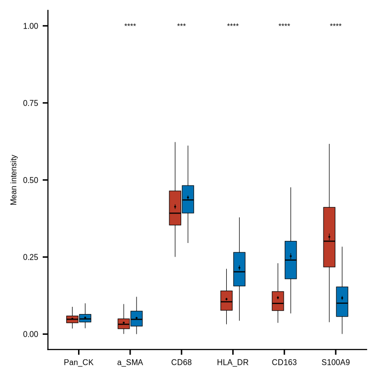
figure7f
mac_markers <- ph_df_markers_norm %>% dplyr::filter(phenotype %in% c("DN_macrophage", "Other_macrophage"))

mac_mean <- mac_markers %>% group_by(roi_id, phenotype) %>%
  dplyr::summarise(S100A9 = mean(S100A9)) %>% ungroup() %>%
  dplyr::mutate(phenotype = case_match(phenotype,
                                       "DN_macrophage" ~ "DN-Mp",
                                       "Other_macrophage" ~ "Other-Mp"))
mac_mean_df <- mac_mean %>% group_by(roi_id) %>%
  dplyr::mutate(n = n()) %>% dplyr::filter(n > 1) %>% ungroup()
mac_mean_df$phenotype <- factor(mac_mean_df$phenotype, levels = c("DN-Mp", "Other-Mp"))

p <- ggplot(mac_mean_df, aes(phenotype, S100A9)) +
  geom_violin(aes(color = phenotype), trim = F,
              linewidth = .3) +#, bounds = c(0,0.3)) +
  geom_boxplot(aes(fill = phenotype), width = .1, show.legend = FALSE,
               outlier.shape = NA, linewidth = .2, color = "black") +
  stat_summary(fun.data = "mean_se", geom = "pointrange", show.legend = F,
               position = position_dodge(.12), size = .025, color = "black") +
  scale_fill_manual(values = c("DN-Mp" = "#BC3C29FF", "Other-Mp" = "#0072B5FF")) +
  scale_color_manual(values = c("DN-Mp" = "#BC3C29FF", "Other-Mp" = "#0072B5FF")) + #ylim(0, 0.35) +
  ylab(glue::glue("Mean intensity of S100A9")) +
  stat_compare_means(aes(label = after_stat(p.signif)),
                     method = "wilcox.test", label.x.npc = "center",
                     size = 1.5, label.y = 0.9,
                     tip.length = 0, bracket.size = 0.1) +
  theme_bmbdc() +
  theme(title = element_text(size = 6),
        axis.ticks = element_line(colour = "black"),
        axis.title.y = element_text(size = 6),
        axis.text.y = element_text(size = 6, colour = "black"),
        axis.title.x = element_blank(),
        axis.text.x = element_text(size = 6, colour = "black"),
        axis.line.x = element_line(linewidth = 0.4),
        axis.line.y = element_line(linewidth = 0.4),
        legend.position="none")
ggsave(glue::glue("{res_dir}/fig7f_polaris_mac_S100A9_intensity_boxplot.pdf"), p, height = 3, width = 3)
p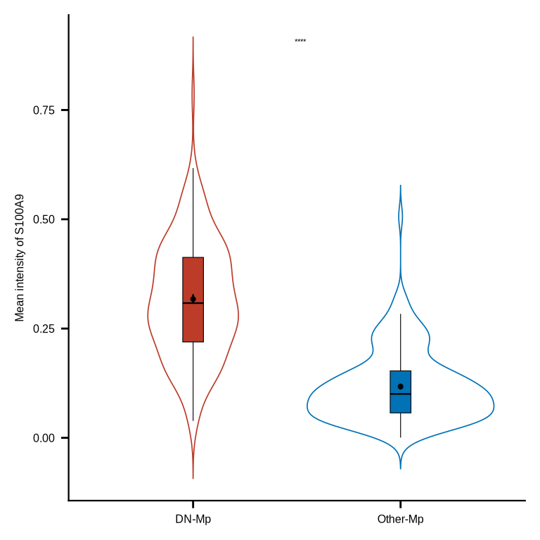
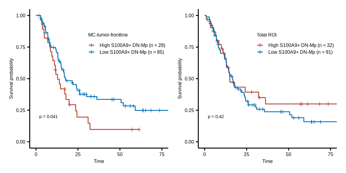
figure7g
s100a9_mac_group <- readr::read_csv(glue::glue("{dat_dir}/polaris_s100a9_mac_meta.csv"))
os_df <- readr::read_csv(glue::glue("{dat_dir}/polaris_os_info.csv"))

#TB
mac_prop <- s100a9_mac_group %>% group_by(sample_name, core_id, s100a9_group, meta_cl) %>%
  dplyr::summarise(nc = n()) %>% group_by(sample_name, core_id, meta_cl) %>%
  dplyr::mutate(nt = sum(nc), prop = nc/nt, s100a9_group = as.factor(s100a9_group)) %>%
  tidyr::complete(s100a9_group, fill = list(prop = 0)) %>% ungroup()

s100a9_mac_prop <- mac_prop %>% dplyr::filter(s100a9_group %in% "S100A9+ DN-Mp" & meta_cl %in% "TB") %>%
  left_join(os_df, by = c("sample_name", "core_id" = "core"))

s100a9_mac_os <- s100a9_mac_prop %>% dplyr::filter(neo_chemo == 0) %>%
  dplyr::mutate(group_43 = case_when(prop >= quantile(prop, probs = 0.75) ~ "High S100A9+ DN-Mp (n = 28)",
                                     prop < quantile(prop, probs = 0.75) ~ "Low S100A9+ DN-Mp (n = 85)"))

grid.draw.ggsurvplot <- function(x){
  survminer:::print.ggsurvplot(x, newpage = FALSE)
}

psurvx <- ggsurvplot(surv_fit(Surv(os_month, os_state) ~ group_43, data = s100a9_mac_os),
                     palette = c("High S100A9+ DN-Mp (n = 28)" = "#BC3C29FF", "Low S100A9+ DN-Mp (n = 85)" = "#0072B5FF"),
                     size = 0.5, censor.size = 3, pval.size = 2,
                     pval = T, risk.table = F, xlim = c(0,75),
                     legend.labs = levels(droplevels(as.factor(unlist(s100a9_mac_os[, "group_43"])))))
psurvx$plot <- psurvx$plot +
  guides(color=guide_legend(title="MC-tumor-frontline")) +
  theme(axis.title.y = element_text(size = 6),
        axis.text.y = element_text(size = 6),
        axis.title.x = element_text(size = 6),
        axis.text.x = element_text(size = 6),
        legend.text = element_text(size = 6),
        legend.title = element_text(size = 6),
        legend.position = c(0.7,0.75),
        legend.key.size = unit(0.1, 'cm'))

ggsave(glue::glue("{res_dir}/fig7g_polaris_S100A9_DNmac_propDNmac_os_nochemo_g43_TB.pdf"),
       plot = psurvx, width = 3, height = 3)


#Total
mac_prop <- s100a9_mac_group %>% group_by(sample_name, core_id, s100a9_group) %>%
  dplyr::summarise(nc = n()) %>% group_by(sample_name, core_id) %>%
  dplyr::mutate(nt = sum(nc), prop = nc/nt, s100a9_group = as.factor(s100a9_group)) %>%
  tidyr::complete(s100a9_group, fill = list(prop = 0)) %>% ungroup()

s100a9_mac_prop <- mac_prop %>% dplyr::filter(s100a9_group %in% "S100A9+ DN-Mp") %>%
  left_join(os_df, by = c("sample_name", "core_id" = "core"))

s100a9_mac_os <- s100a9_mac_prop %>% dplyr::filter(neo_chemo == 0) %>%
  dplyr::mutate(group_43 = case_when(prop >= quantile(prop, probs = 0.75) ~ "High S100A9+ DN-Mp (n = 32)",
                                     prop < quantile(prop, probs = 0.75) ~ "Low S100A9+ DN-Mp (n = 91)"))

psurvy <- ggsurvplot(surv_fit(Surv(os_month, os_state) ~ group_43, data = s100a9_mac_os),
                     palette = c("High S100A9+ DN-Mp (n = 32)" = "#BC3C29FF", "Low S100A9+ DN-Mp (n = 91)" = "#0072B5FF"),
                     size = 0.5, censor.size = 3, pval.size = 2,
                     pval = T, risk.table = F, xlim = c(0,75),
                     legend.labs = levels(droplevels(as.factor(unlist(s100a9_mac_os[, "group_43"])))))
psurvy$plot <- psurvy$plot +
  guides(color=guide_legend(title="Total ROI")) +
  theme(axis.title.y = element_text(size = 6),
        axis.text.y = element_text(size = 6),
        axis.title.x = element_text(size = 6),
        axis.text.x = element_text(size = 6),
        legend.text = element_text(size = 6),
        legend.title = element_text(size = 6),
        legend.position = c(0.7,0.75),
        legend.key.size = unit(0.1, 'cm'))
ggsave(glue::glue("{res_dir}/fig7g_polaris_S100A9_DNmac_propDNmac_os_nochemo_g43_Total.pdf"),
       plot = psurvy, width = 3, height = 3)

psurvx$plot | psurvy$plot